Unveiling the Black Box

.title[
# Unveiling the Black Box
]
.subtitle[
## Researching Algorithms with Audit Studies
]
.author[
### <b>Fabio Votta</b> <i>(University of Amsterdam)</i>
]
.date[
###  <svg viewBox="0 0 512 512" style="height:1em;position:relative;display:inline-block;top:.1em;fill:black;" xmlns="http://www.w3.org/2000/svg"> <path d="M326.612 185.391c59.747 59.809 58.927 155.698.36 214.59-.11.12-.24.25-.36.37l-67.2 67.2c-59.27 59.27-155.699 59.262-214.96 0-59.27-59.26-59.27-155.7 0-214.96l37.106-37.106c9.84-9.84 26.786-3.3 27.294 10.606.648 17.722 3.826 35.527 9.69 52.721 1.986 5.822.567 12.262-3.783 16.612l-13.087 13.087c-28.026 28.026-28.905 73.66-1.155 101.96 28.024 28.579 74.086 28.749 102.325.51l67.2-67.19c28.191-28.191 28.073-73.757 0-101.83-3.701-3.694-7.429-6.564-10.341-8.569a16.037 16.037 0 0 1-6.947-12.606c-.396-10.567 3.348-21.456 11.698-29.806l21.054-21.055c5.521-5.521 14.182-6.199 20.584-1.731a152.482 152.482 0 0 1 20.522 17.197zM467.547 44.449c-59.261-59.262-155.69-59.27-214.96 0l-67.2 67.2c-.12.12-.25.25-.36.37-58.566 58.892-59.387 154.781.36 214.59a152.454 152.454 0 0 0 20.521 17.196c6.402 4.468 15.064 3.789 20.584-1.731l21.054-21.055c8.35-8.35 12.094-19.239 11.698-29.806a16.037 16.037 0 0 0-6.947-12.606c-2.912-2.005-6.64-4.875-10.341-8.569-28.073-28.073-28.191-73.639 0-101.83l67.2-67.19c28.239-28.239 74.3-28.069 102.325.51 27.75 28.3 26.872 73.934-1.155 101.96l-13.087 13.087c-4.35 4.35-5.769 10.79-3.783 16.612 5.864 17.194 9.042 34.999 9.69 52.721.509 13.906 17.454 20.446 27.294 10.606l37.106-37.106c59.271-59.259 59.271-155.699.001-214.959z"></path></svg> favstats.github.io/nefca2023 (Slides) <br>  <svg viewBox="0 0 512 512" style="height:1em;position:relative;display:inline-block;top:.1em;fill:blue;" xmlns="http://www.w3.org/2000/svg"> <path d="M459.37 151.716c.325 4.548.325 9.097.325 13.645 0 138.72-105.583 298.558-298.558 298.558-59.452 0-114.68-17.219-161.137-47.106 8.447.974 16.568 1.299 25.34 1.299 49.055 0 94.213-16.568 130.274-44.832-46.132-.975-84.792-31.188-98.112-72.772 6.498.974 12.995 1.624 19.818 1.624 9.421 0 18.843-1.3 27.614-3.573-48.081-9.747-84.143-51.98-84.143-102.985v-1.299c13.969 7.797 30.214 12.67 47.431 13.319-28.264-18.843-46.781-51.005-46.781-87.391 0-19.492 5.197-37.36 14.294-52.954 51.655 63.675 129.3 105.258 216.365 109.807-1.624-7.797-2.599-15.918-2.599-24.04 0-57.828 46.782-104.934 104.934-104.934 30.213 0 57.502 12.67 76.67 33.137 23.715-4.548 46.456-13.32 66.599-25.34-7.798 24.366-24.366 44.833-46.132 57.827 21.117-2.273 41.584-8.122 60.426-16.243-14.292 20.791-32.161 39.308-52.628 54.253z"></path></svg> favstats <br>  <svg viewBox="0 0 448 512" style="height:1em;position:relative;display:inline-block;top:.1em;fill:#615ff7;" xmlns="http://www.w3.org/2000/svg"> <path d="M433 179.11c0-97.2-63.71-125.7-63.71-125.7-62.52-28.7-228.56-28.4-290.48 0 0 0-63.72 28.5-63.72 125.7 0 115.7-6.6 259.4 105.63 289.1 40.51 10.7 75.32 13 103.33 11.4 50.81-2.8 79.32-18.1 79.32-18.1l-1.7-36.9s-36.31 11.4-77.12 10.1c-40.41-1.4-83-4.4-89.63-54a102.54 102.54 0 0 1-.9-13.9c85.63 20.9 158.65 9.1 178.75 6.7 56.12-6.7 105-41.3 111.23-72.9 9.8-49.8 9-121.5 9-121.5zm-75.12 125.2h-46.63v-114.2c0-49.7-64-51.6-64 6.9v62.5h-46.33V197c0-58.5-64-56.6-64-6.9v114.2H90.19c0-122.1-5.2-147.9 18.41-175 25.9-28.9 79.82-30.8 103.83 6.1l11.6 19.5 11.6-19.5c24.11-37.1 78.12-34.8 103.83-6.1 23.71 27.3 18.4 53 18.4 175z"></path></svg> <a href="mailto:favstats@fosstodon.org" class="email">favstats@fosstodon.org</a> <br>  <svg viewBox="0 0 448 512" style="height:1em;position:relative;display:inline-block;top:.1em;fill:#0085ff;" xmlns="http://www.w3.org/2000/svg"> <path d="M400 32H48C21.5 32 0 53.5 0 80v352c0 26.5 21.5 48 48 48h352c26.5 0 48-21.5 48-48V80c0-26.5-21.5-48-48-48z"></path></svg> favstats                                                                          April 8 2024 - AlgoSoc YSN Spring School
]

---

---

## What is an algorithm audit study?

.font150["an <b>.gold[empirical study]</b> investigating a <b>.darkblue[public]</b> <b>.orange[algorithmic system]</b> for potential <b>.purple[problematic behavior]</b>"  (Bandy 2021)]

</center>

+ <b>.gold[empirical study]</b>

+ includes an experiment or analysis (quantitative or qualitative)
  
--
  
+ <b>.darkblue[public]</b> (optional?)

+ used in a commercial context or other public setting such as law enforcement, education, criminal justice, or public transportation

+ <b>.orange[algorithmic system]</b>

+ socio-technical system influenced by at least one algorithm
  
--
  
+ <b>.purple[problematic behavior]</b>

+ discrimination, distortion, exploitation, or misjudgement. 
  + A behavior is problematic when it *causes harm* (or potential harm)

---

## How to conduct an algorithm audit study? .font50[(Bandy 2021; Urman et al. 2024)]

+ <b>Code audit</b>

+ researchers obtain and analyze the code that makes up the algorithm
  
  + *rarely available*
  
  > Weber & Kosterich 2018: "Investigates code of 59 open source mobile news apps"
  
  + "Much of the code that automates news distribution is created separately from the journalism world."

]

![](img/codecode.jpg)

]

---

## How to conduct an algorithm audit study? .font50[(Bandy 2021; Urman et al. 2024)]

+ Code audit

+ <b>direct/non-personalized scraping</b>

+ using APIs / webscraping
  
  + *limited usefulness because results are not personalized*

> *"Foreign beauties want to meet you": The sexualization of women in Google’s organic and sponsored text search results*  Urman & Makhortykh (2023)
  
    + "We find evidence of the sexualization of women, particularly those from the Global South and East, in search outputs in both organic and sponsored search results."

]

![](https://encrypted-tbn0.gstatic.com/images?q=tbn:ANd9GcRWp4SHWSUXCi88mAamdLNMpt6tRygt_XRdV5DywbOGtA&s)

]

---

## How to conduct an algorithm audit study? .font50[(Bandy 2021; Urman et al. 2024)]

+ Code audit

+ direct/non-personalized scraping

+ <b>Sock puppet/personalized scraping</b>

+ creating accounts/entities that receive personalized recommendations
  
  + *carrier puppets/repurposing*: impersonated users affect the real-world system and may "carry" effects onto end users
  
  + research has (in-)direct effects on algorithmic system
  
  > Hagar & Diakopoulos (2023)
  
  + "We find almost no evidence of proactive news exposure on TikTok’s behalf."

]

![](https://upload.wikimedia.org/wikipedia/commons/thumb/0/0b/Sock_puppet_and_keyboard.jpg/640px-Sock_puppet_and_keyboard.jpg)

]

---

## How to conduct an algorithm audit study? .font50[(Bandy 2021; Urman et al. 2024)]

+ Code audit

+ direct/non-personalized scraping

+ Sock puppet/personalized scraping

+ <b>Crowdsourcing</b>

+ researchers collect data by hiring end users to test the algorithm
  
  >  Glaesener (2022) Exploring Siri’s Content Diversity Using a Crowdsourced Audit. 
  
  + "A diverse sample of 170 US-based Siri users between the ages of 18-64 performed five identical queries about politically controversial issues.  Forty-two percent of the participants received the six most frequent answers, while 22% of the users received unique answers."

]

![](https://sloanreview.mit.edu/wp-content/uploads/2017/05/MAG-Malhotra-Internal-Crowdsourcing-1200-1200x630.jpg)

]

---

# The Role of Algorithms

# in Digital Political Advertising

![](https://media3.giphy.com/media/3o6Yg4GUVgIUg3bf7W/giphy.gif)

*studying ad delivery algorithms by "expert"sourcing*

---

### The Role of Algorithms in Digital Political Advertising

*The explicit assumption here that advertisers typically have strong control over who sees which ad*

]

**But there is more than *just* targeting criteria that decides who sees political ads:**

+ advertisers can set targeting *boundaries*

+ *ad delivery algorithms* "decide" which individual users get ads from which advertiser

+ they do this by organizing *automated ad auctions* which set prices

]

---

### Who decides who sees which ad on Meta?

+ **Ad auctions** = an auction takes place that determines which ad by whom is shown

---

### Who decides who sees which ad on Meta?

+ **Relevance** = how relevant is the ad to the user

[(Meta Business Help Center, 2022)](https://www.facebook.com/business/help/430291176997542)

---

### Who decides who sees which ad on Meta?

+ **Ad auctions** = an auction takes place that determines which ad by whom is shown: based on *budget*

+ **Relevance** = how relevant is the ad to the user

---

### A (silly) example

.pull-left[
    <img src="https://images-na.ssl-images-amazon.com/images/S/compressed.photo.goodreads.com/books/1465341854i/12111823.jpg" width = "6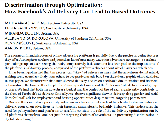0%">
]

---

### Prior Research (Ali et al., 2020,2021)

---

### Prior Research (Ali et al., 2020,2021)

When targeting the same audience, at the same time, with the same budget:

+ Ad delivery is heavily skewed along gendered and racial stereotypes
  + even without the intent of the advertiser [(Ali et al. 2020)](https://dl.acm.org/doi/10.1145/3359301)

Images invisible to humans but still detectable by algorithm:

+ yield **similar skews** in delivery

+ highlights importance of algorithm

+ less based on differences in user behavior/preferences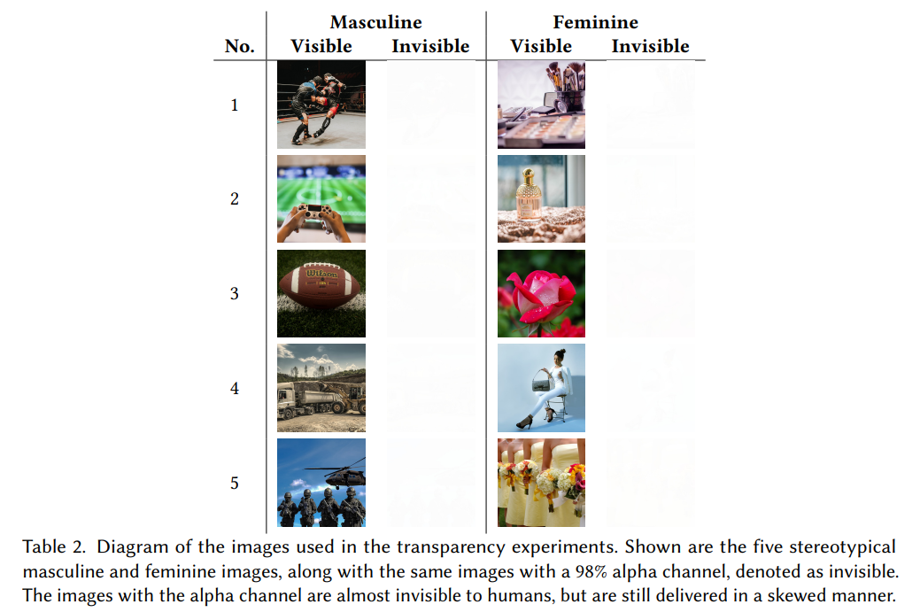
]

---

### Prior Research (Ali et al., 2020,2021)

When targeting the same audience, at the same time, with the same budget:

Regarding political ads [(Ali et al., 2021)](https://dl.acm.org/doi/pdf/10.1145/3437963.3441801):

+ Political ads more often delivered to ideologically congruent audience
      + Bernie ads → higher % D;
      + Trump ads → higher % R

+ **Increased cost**

+ Liberal ad to a liberal audience: *21 Dollar per 1000 users*;
  + Conservative ad delivered to liberal audience: *40 Dollar per 1000 users*.
]

+ when tricking Facebook into classifying non-partisan ads as partisan

]

---

## Research Question

### How does the Meta ad delivery algorithm<br>influence the pricing & distribution of political ads<br>in the Netherlands?

---

# Research Design

---

### Research Design

+ Algorithm audit study

+ Place the same ads targeting the same audiences (9 different ones)

+ Collaborate with Dutch parties to place political ads

+ Final collaboration with 3:

1. GroenLinks (Green party)
  2. VVD (centre-right party of PM Rutte)
  3. PvdA (social democrats)

---

### Hypotheses

![](img/relevant_quote.png)

[(Meta Business Help Center, 2022)](https://www.facebook.com/business/help/430291176997542)

> **H1:** **The more relevant** an audience is for an ad, **the cheaper is the cost** for reaching 1000 users in that audience.

We expect that ads by party with a greater share of supporters are less expensive (H2)

> **H2:** Parties with a greater share of supporters pay less for reaching 1000 users.

---

# Ad Creative and Setup

---

## How the ad looked like on Desktop

---

## How the ad looked like on Desktop

---

## Results

---

### Between-party differences

`\(\rightarrow\)` we consistently find one party that pays less and reaches more people

---

#### Between-party differences (per individual ad)

.font80[PvdA pays the least (**10-12 cents less** or: 9-11%) & reaches more people (~**1.1 - 1.3k more** per ad)]

```
## # A tibble: 15 × 5
##    party      reach share targeting        relevance
##    <chr>      <dbl> <dbl> <chr>                <dbl>
##  1 PvdA       13138  52.1 Higher Education         1
##  2 PvdA       12917  51.7 Higher Education         1
##  3 GroenLinks 11938  51.7 Higher Education         2
##  4 VVD        11528  51.6 Higher Education         1
##  5 VVD        11845  51.6 Higher Education         1
##  6 GroenLinks 11622  51.6 Higher Education         2
##  7 PvdA       12860  51.6 Higher Education         1
##  8 GroenLinks 11727  51.4 Higher Education         2
##  9 PvdA       12729  51.1 Higher Education         1
## 10 GroenLinks 11486  51.1 Higher Education         2
## 11 VVD        11388  51.0 Higher Education         1
## 12 PvdA       12632  50.9 Higher Education         1
## 13 GroenLinks 11509  50.9 Higher Education         2
## 14 VVD        11344  50.8 Higher Education         1
## 15 VVD        11260  50.6 Higher Education         1
```

]

]

---

#### Between-party differences (per target audience)

---

### Within-party differences

---

### Within-party differences - Price per 1k

Ads **cost less for**:

+ *higher-educated* vs. *lower-educated audience*

Ad price **does not statistically differ for**:

+ Audience *interested in the economy* vs. *not interested*

+ Audience *interested in politics* vs. *not interested*

Ads **cost more for**:

+ Audience *interested in the environment* vs. *not interested*

]

![](img/diffs1.png)

]

---

**18-24 year olds and women are reached less (and cost more to reach)**

![](img/priceshare.png)

---

# Algorithms are a black box

+ It takes considerable effort to study them

+ they behave in ways that can be quite unexpected

+ yet with *algorithm audit study* we can start understanding their outcomes

---

# Curious to learn more?

I am currently in the process of building on this research by conducting a very similar design during the European Parliament elections

+ 10 countries + European Level

+ 16 parties confirmed

+ 18 parties still considering offer

---

## Thank you for your attention! Questions?

Link to presentation: *favstats.github.io/algosoc-spring24*

![](https://c.tenor.com/Q9qk5zN5EesAAAAM/space-kitten.gif)
![](https://c.tenor.com/Q9qk5zN5EesAAAAM/space-kitten.gif)

]

![](https://c.tenor.com/Q9qk5zN5EesAAAAM/space-kitten.gif)
![](https://c.tenor.com/Q9qk5zN5EesAAAAM/space-kitten.gif)

]

---

## Literature

Weber, M. S., & Kosterich, A. (2018). Coding the News: The role of computer code in filtering and distributing news. Digital Journalism, 6(3), 310–329. https://doi.org/10.1080/21670811.2017.1366865

---

## Appendix

---

## Four .fancy[Types] of Problematic Behavior .font50[(Bandy 2021)]

**1. Discrimination**

disparate treatment based on race, age, gender, location, socio-economic status, or intersecting identities 
  
> Example: showing high-paying job ads primarily to men; facial recognition systems performing poorly on minority groups
  
]

---

## Four .fancy[Types] of Problematic Behavior

**1. Discrimination**

Outcomes distort or obscure reality

> Example: Search engines reinforcing stereotypes; filter bubbles

]

**3. Exploitation**

Inappropriate use of (sensitive) personal information
  
> Example: Inferring sensitive personal information without consent

]

---

## Four .fancy[Types] of Problematic Behavior

**1. Discrimination**

Outcomes distort or obscure reality

> Example: Search engines reinforcing stereotypes; filter bubbles

]

**3. Exploitation**

Inappropriate use of (sensitive) personal information
  
> Example: Inferring sensitive personal information without consent	
  
  
**4. Misjudgment**

The algorithm makes incorrect predictions or classifications.

> Example: Algorithms incorrectly categorizing users' employment status or interests; content moderation errors

]

-->

-->

-->

-->

-->

-->

-->

-->

-->

-->

-->

-->

-->

-->